KEY POINTS FROM THIS ARTICLE
— Swing voters are not the same as swing states. This article discusses a metric called “elasticity” for counties, which tracks a county’s variance in vote margin, to help us better identify and draw the distinction between these two.
— In the 2020 election, Republicans face an extremely tough challenge in holding Wisconsin, as the highly elastic nature of the state, combined with the heavily Democratic environment, open up too many holes to cover in order to maintain their 2016 margins. Similarly, Arizona may be difficult to hold for the GOP, given the leftward lurch of Maricopa County.
— In inelastic states like Florida and North Carolina, both parties are heavily reliant on turnout from their bases in order to carry the state. Biden’s strength, however, may be in his ability to more closely match Barack Obama’s performance in the Republican areas of the states, which are generally more elastic than the Democratic areas.
Introduction
The concept of a “swing state” is thought to be an easily-understood notion in politics — it’s a state that could tip either way in any given election. But not every voter in a swing state is actually a swing voter, and it’s important to draw the distinction. Some states, like Wisconsin, do have a lot of actual swing voters. But other swing states, like Florida and North Carolina, are home to relatively few swing voters. The closely contested nature of these states comes instead from a relatively equal set of committed partisans on each side, and election victories in such states generally go to the candidate that can turn out the most voters on their side.
This is a tough thing to measure, however — how can we understand which category certain states fall into? One thing we can examine is the tendency for the state’s counties to swing between parties across elections.
For example, a county could vote for the Republican by a five-point margin for governor and vote for the Democrat by a 10-point margin for president, indicating a high degree of openness to voting for any candidate, regardless of party. Examining this tendency should thus help us gauge the partisan loyalty of a county’s voters across offices and would thus provide a rough, but vote-based estimate of the types of voters in an area and their electoral “elasticity.” With context, this would greatly help us in identifying how persuadable voters in counties really are.
Understanding and quantifying the elasticity of voters in areas (a concept discussed by Nate Silver at FiveThirtyEight) is an extremely important thing for candidates, as it helps them decide on resource allocation and helps in setting campaign strategy for maximizing the ultimate number: votes. For example, Joe Biden would likely be wasting his time airing ads about bipartisanship in a place like Florida’s Broward County, a Democratic stronghold whose voters are already fairly entrenched in their views. But he might be better off airing those ads in Wisconsin, where more swing voters exist, and investing in a heavy turnout machine in Broward County to turn out his voting base instead.
To measure this tendency, we’ll introduce a concept called “elasticity” for counties. This concept measures the deviations in a county’s percentage-based vote margin across a set of elections, which we use as a proxy for the openness of a county’s voters to voting for candidates across the political spectrum, regardless of political affiliation.
It is important to note that what this metric measures is the vote-based electoral “bipartisanship” of counties across offices — i.e. “How much has this county’s vote varied across elections?” This is different from the concept of “swing counties.” You can imagine a county being fairly elastic as it oscillates between R+20 and R+50, while being reliably red — we see that a fair amount of voters are open to voting for the Democrat, even if the county appears to be solidly Republican in each of those hypothetical elections. In a closely-contested election, those margins can make all the difference.
The metric is computed as follows: For any set of elections {A, B, C, D, …}, we plot the (Republican, Democratic) vote by county on an (x, y) coordinate scale and compute the pairwise Euclidean distance between all points. These distances are then all summed to obtain an elasticity score for the county. Basically, the more distance between the points, the more elastic the county is, because that means there’s been more variance in how the county has voted in recent elections.
In this column, our set of elections will consist of the most recent Senate election, the most recent governor election, and the two most recent presidential elections. We will be analyzing four closely-watched states in this year’s presidential election: Wisconsin, Florida, Arizona, and North Carolina. The elasticity of a county will be denoted by (E number), and we will have five tiers: very inelastic (E < 15), moderately inelastic (E 15-25), slightly elastic (E 25-40), moderately elastic (E 40-60), and highly elastic (E > 60).
Let’s explore this in more detail by looking at the elasticity metrics of two counties: Vernon County in Wisconsin (a moderately elastic area), and Pinellas County in Florida (a moderately inelastic one).
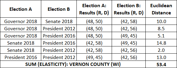
Let’s first collect the set of results we need to calculate Vernon County’s elasticity, with the vote for each election represented in (Republican, Democrat) format. For ease of viewing, we will round results to the nearest whole number.
The 2018 governor results were (48% Republican, 50% Democratic), the 2018 Senate results were (42, 58), the 2016 presidential results were (49, 45), and the 2012 presidential results were (42, 56). We will now calculate the pairwise Euclidean distance between all these points and sum them up to get the elasticity of the county, as shown in the table below. For information on how the two-dimensional Euclidean distance used is calculated, we recommend taking a quick glance here.
Table 1: Elasticity of Vernon County, Wisconsin
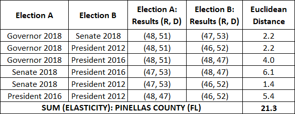
The elasticity of Vernon County becomes especially clear when contrasted with that of a county like Pinellas in Florida, which has a far less variable vote margin between elections.
Table 2: Elasticity of Pinellas County, Florida
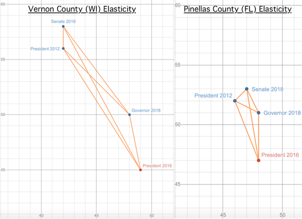
We can also contrast the elasticity of two counties with the visual below — essentially, elasticity is the sum of the edge lengths in a graph that connects all four points, plotted by (R, D) vote percentages on the (x, y) coordinate plane, with each other. The longer the edges, the more elastic the county is. Thus, an elastic county would have a “stretchier” shape, as the set of vertices would be farther apart.
Table 3: Elasticity of Vernon County, WI vs. Pinellas County, FL
With that explanation out of the way, let’s look at some of these key states.
Wisconsin
Map 1: Wisconsin elasticity by county, 2012-2018
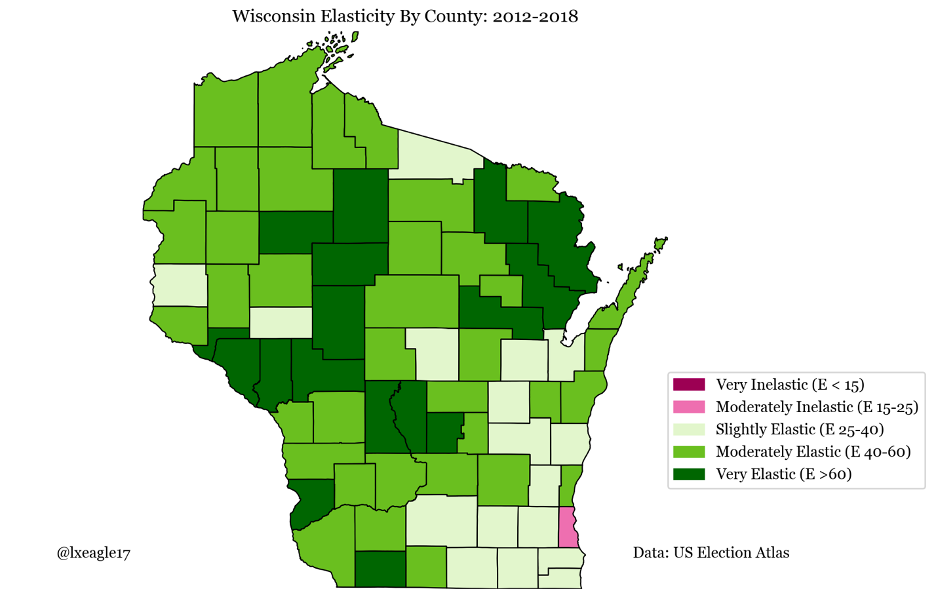
Wisconsin is the classic example of a traditional swing state: one comprised of moderate swing voters who swing between parties based on candidacies and the national mood. Trump’s 2016 victory in Wisconsin was by the slimmest of margins (less than 25,000 votes), and even the most minor swing away could spell doom for him. However, an unfavorable national environment and the highly elastic nature of the state in many of Trump’s 2016 counties bode for some serious trouble — in such an environment, one can reasonably expect the president to sustain some losses in elastic areas like western and northeastern Wisconsin — counties like Marinette (E 73.4) and Trempealeau (E 70.7) are microcosms of the problems the incumbent may face. Republicans must prevent Joe Biden from coming close to Obama’s 2012 margin or to Sen. Tammy Baldwin (D-WI)’s 2018 margins if they hope to carry the state.
The Democratic counties of Dane (E 33.0) and Eau Claire (E 37.4) do have some degree of elasticity, but there is reason to believe that this is cause for Republican concern rather than celebration. Recall that elasticity gives us a proxy for the possibility of divergence from the average — this is to say, if a county is normally 15 points Democratic but with an elasticity of 50, the margin may rise or fall by a fair amount in either direction.
The problem? There is reason to believe that Democrats underperformed here in 2016 relative to what we can expect in 2020, and that the high elasticity of this state indicates a fair amount of room to grow for the party. The elasticity of these areas is largely due to the sharp Democratic improvement in 2018, showing that more latent Democratic votes exist than previously thought possible. For example, while Clinton won Eau Claire and Dane by 7 and 47 points, respectively, now-Gov. Tony Evers (D) won them by 12 and 51, and Baldwin by 22 and 55. In a national environment that more closely mirrors 2018 than 2016, it is reasonable to expect that the voters who swung from Trump to Baldwin/Evers may stick with that switch.
Republican problems in the state are further compounded by the problems they may face with keeping votes in the suburbs. Racine (E 30.0) and Kenosha (E 37.5), both counties Obama won in 2012, were won by Trump in 2016, but Baldwin won them in 2018, and they are elastic enough to allow for further erosion among Trump’s base. The Waukesha (E 33.7), Washington (E 30.0), and Ozaukee (E 42.7) counties (WOW counties) are elastic enough to the point where Republicans could see losses of two to three percentage points in margin compared to 2016 — in fact, this would mirror Tammy Baldwin’s 2018 victory and build on signs seen in Jill Karofsky’s 2020 Supreme Court victory (Karofsky won as a Democratic-backed candidate in a technically nonpartisan race).
Such a margin may seem small, but it is, in fact, one of the biggest red flags for the party in 2020; a moderately elastic area with 350,000 votes is far more dangerous to a statewide margin than a highly elastic area with 40,000 votes simply due to the sheer volume of votes in the former. If just 4% of voters swung away from Trump’s 2016 margin in the WOW counties, the Democrats would carry the state by merely maintaining their margins elsewhere.
Because of the national environment, however, continued improvement in the WOW counties combined with Democrats regaining the ground they lost in 2016 in western Wisconsin is an entirely plausible scenario.
Florida
Map 2: Florida elasticity by county, 2012-2018
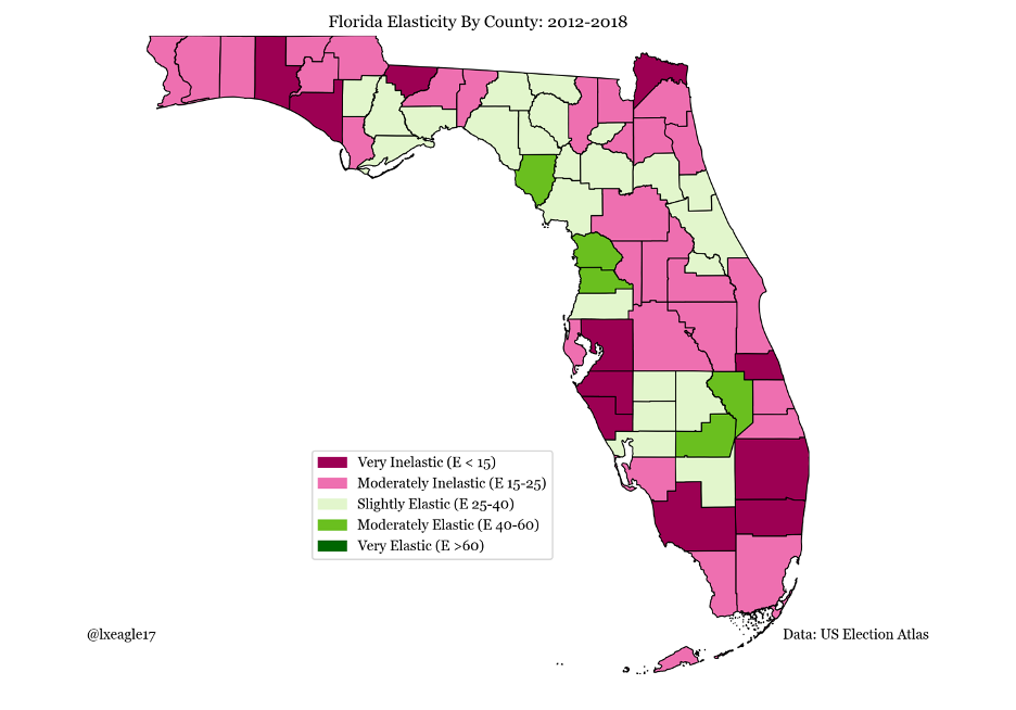
Florida is the perfect example of a turnout-based swing state. In a state like this, swing voters are actually relatively sparse, and statewide control goes to the party with the better organizing and ground game.
Notice that elasticity tells us the proportion of voters in a county that have shown an openness to voting for either party across elections. This gives us a proxy for how reliable a party’s support base is and whether they can expect any defections from their expected strength across the set of elections. This is especially important for a state as closely contested as this one.
In Florida, the Democrats would be gladdened to see that their support bases in Broward (E 11.2) and Miami-Dade (E 21.3) are very and moderately inelastic, respectively. This means that their support is locked in and that there is little room for them to fall in these areas. Obama won the state twice thanks to an incredibly strong turnout machine that brought base voters to the polls in droves, and Biden will seek to replicate that.
The Republicans, however, cannot feel as safe. The Florida Panhandle, a reliably Republican area, is one of the more elastic parts of this turnout-based state, and the trio of counties above Tampa Bay (Pasco, Hernando, and Citrus) are fairly elastic counties that are generally double-digit Republican strongholds — in fact, Hernando (E 46.3) and Citrus (E 41.1) are two of the five most elastic counties in Florida. If Biden is able to siphon away a significant amount of votes from these areas, holding the state would become an incredibly tall ask for Republicans.
North Carolina
Map 3: North Carolina elasticity by county, 2012-2018
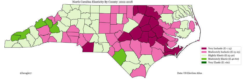
Another turnout-based swing state, North Carolina is a state that skews more Republican than the rest of the nation, but with enough Democratic voters to stay competitive. Flipping this state will be the tallest order for Democrats in 2020; however, it is once again important to note that the traditionally Democratic areas in central, southern, and northeastern North Carolina are far less elastic than the Republican base in the southeastern and western part of the state. Outside of the eastern part of the state, the only truly elastic county is Robeson County (E 53.8) — despite being a historically Democratic stronghold, Trump managed to win the county by four percentage points only four years after Obama carried it by 18.
However, although Democrats can expect to regain a fair amount of the ground lost in 2016 in these areas under the current national environment, flipping the state on swing voters alone in these areas will be a nigh-impossible task. Although a bluer-than-usual national environment may help them along the way, flipping North Carolina is a tougher task for Democrats and will rely on them turning out their voting base in the counties of Wake (E 29.7), Guilford (E 21.8), and Cumberland (E 15.3), and continuing the swing of suburban voters in Wake County (one of the few populous areas with any elasticity for them to capitalize on).
Arizona
Map 4: Arizona elasticity by county, 2012-2018
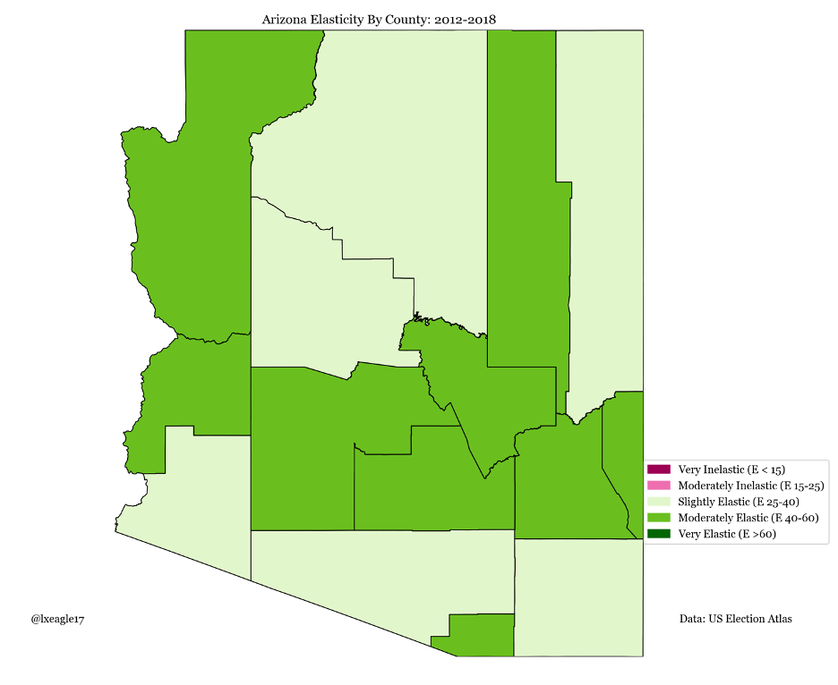
Arizona falls in the middle of the spectrum of states we are analyzing — although it is nowhere near as elastic as Wisconsin, it is certainly more elastic than Florida.
Pinal (E 47.3) and Maricopa (E 46.9) are the two most interesting counties to examine. Traditionally Republican, the high elasticity of these counties would be a source of concern for several Republicans, as they can ill-afford to lose too many votes here if they wish to hang on to the state at the Senate and presidential levels. Maricopa, in particular, is home to Phoenix and its suburbs and cast more than 1.5 million votes in 2016. The county includes significant pockets of white college-educated voters, a group that Biden has been making gains with in polls.
The exceptionally high elasticity of Maricopa, when combined with the sheer volume of voters present, makes this a particularly appealing target county for Democrats, as investment here could flip an incredibly high amount of voters, and Kyrsten Sinema used this to great effect in her 2018 Senate victory over Martha McSally. Conversely, a popular Republican incumbent with high approval ratings could see a victory like Gov. Doug Ducey’s double-digit win in the 2018 gubernatorial race; however, with current trends, this is increasingly unlikely for Republicans, meaning their focus needs to be on stemming the bleed of swing voters instead.
Conclusion
Elasticity is a metric that helps us quantify the voting nature of states and the reliability of a support base. We can see through this metric that states like Florida are turnout-based and have relatively little divergence in voting margins between elections on a county-level basis, implying a relative lack of swing voters. Meanwhile, states like Wisconsin are highly elastic, indicating the presence of swing voters that must be won over in order to carry the state. In conjunction with electoral trends and context, elasticity helps us gauge the possibility of latent votes for either party in the 2020 election and helps identify key areas that campaigns must target to carry the state.
| Lakshya Jain is a software engineer who recently graduated from UC Berkeley with a Masters’ in Computer Science, with a focus on machine learning. His data-centric background and political interest led him to analyze elections in his spare time. More of his analyses can be found at politicalsalad.com or on Twitter @LXEagle17. |