KEY POINTS FROM THIS ARTICLE
— The Trial-Heat and Convention Bump Forecasting Models have an excellent record for accurate predictions of the presidential elections going back to 1992.
— Forecasting models depend on applying electoral history to the current election, but 2020 is historically abnormal (at least, in the period since 1948).
— The greatest challenge for forecasting this year is in how the catastrophic second quarter GDP should be treated.
— Based on President Trump’s approval ratings, in general and on the economy, as well as the projected third quarter GDP growth rates, the forecasts should depend exclusively on the preference polls, and they point to another extremely close election.
The forecasting models
Entering the home stretch of this surreal presidential election between President Donald Trump and former Vice President Joe Biden, many of us are holding our breath and looking with anxiety and trepidation toward Election Day. This forecast analysis will not alleviate this angst, but might prepare us a bit for what we may be heading toward.
The basis for my presidential forecast is the Trial-Heat and Economy forecasting model. It is a simple, intuitively sensible, historically grounded, and transparent forecasting equation with a long history of accurate forecasts of the national two-party popular vote for president.
First developed and published in 1990 (with Ken Wink), it was first used in the 1992 election and predicted Bill Clinton’s win. Apart from a few tweaks to the model over the years, it remains substantially as originally devised, a sophisticated reading of the preference polls set in their context and informed by their historical association with the national popular two-party vote. The forecast equation is estimated by a regression analysis of two predictor variables: The in-party’s (president’s party) share of support in the preference polls available 60 days before the election (around Labor Day at the beginning of September) and the growth rate of the economy in the second quarter of the election year. This is measured by the annualized change in the second quarter GDP as reported by the Bureau of Economic Analysis in its end of August release, with adjustments for incumbency and the diminishing effects of extreme values.
Developed prior to the 2004 election and built from the same perspective as the Trial-Heat model, the Convention Bump model draws on polls at different points in the campaign. Rather than using a single Labor Day poll reading, the Convention Bump model uses the in-party candidate’s standing in the preference polls immediately before the first national party convention of the year and the net “convention bump” for the in-party candidate (the gain or loss in the preference polls from before the first convention to after the second convention). This recognizes that a substantial portion of the poll effects of conventions is ephemeral. Adding this companion model not only allows the convention effects to be properly taken into account, but offers a second check of the Trial-Heat model. Any additional check of models based on so few cases with so few predictor variables is reassuring.
Both models have an impressive record of accuracy. Both were within one point of the two-party vote in both 2012 and 2016. The median absolute errors of the after-the-fact estimated expected votes for elections from 1948 to 2016 are 0.8% for the Trial-Heat equation and 1.1% for the Convention Bump equation.
Even the one election in which these models missed the vote by a wide margin is evidence of their strength. The one “big miss” election was the John McCain-Barack Obama 2008 election with the wholly unanticipated cataclysmic Wall Street meltdown crashing between the forecasts and Election Day. With such a huge and unanticipated disruption, any sound forecasting model should have “missed” that election. Setting aside this one understandably aberrant case, the mean absolute error of the forecasts in actual use (pre-election published) is 1.6% for the Trial-Heat equation (1992-2016) and .8% for the Convention Bump equation (2004-2016).
There is history, and then there is 2020
The often unstated reason structural equation forecasts produce fairly accurate predictions of the national vote well in advance of Election Day is they are based on solid statistical analyses of how fundamental political contexts of elections known in advance of the campaign have normally affected the electorate’s response to the intervening campaign and, ultimately, its vote.
The forecasts work because they are based on history and assume the history of past campaigns and elections is a strong guide to how the next election will turn out. Aside from assumptions that the models are right — well specified and with good measurements of predictors — forecasts assume the election being predicted is, generally speaking, historically normal.
This year has been everything but normal, at least not “normal” by post-1948 history standards (the period used in estimating the equations). The overarching abnormality of 2020 is the COVID-19 pandemic. It has altered everyday life since last March when the nation, like much of the world, went into “lockdown.” Life changed, and that included political life as we knew it.
Conventional campaigning basically stopped for months. National nominating conventions went “virtual.” Even now, events are much more limited, and many would not even consider attending.
A number of states are considering conducting the election through mail-in balloting to avoid congestion at polling places and a turnout decline by those fearing health risks from voting in person (though the presumably more secure established absentee voting system would seem to offer a safe alternative). The pandemic and the public health policies in response to it also changed the nation’s economic life. Businesses and industries were forced to shut down to limit the deadly contagion of the virus. The obvious result was an economic collapse.
Beyond the pandemic abnormalities, the election’s context has been marked by widespread divisive protests about racial inequities in policing. In several cities these protests have led to devastating rioting, looting, and violence — in some cases taking place over many weeks. The lawlessness and disorder problem has intensified the strongly polarized political climate.
2020 versus the forecasts
Much of the abnormal and wild contexts of 2020 can be accommodated in the forecast models through the preference polls. To a great extent, and as they normally do with social conditions, the electorate can evaluate the political responsibilities for dealing with the pandemic and rioting and indicate which candidate it believes can better handle these problems. To this extent, the forecasting equations can be applied as normal.
Other aspects of 2020, however, are not so easily dealt with. The models are estimated using the experience of elections without widespread mail-in balloting, with a substantially less partisan and blatantly hostile press, and with surveys conducted in political climates more tolerant of preferences for either major party candidate. Although the models have been resilient over time, it is uncertain whether they will be to these differences.
Restrained early campaigning and the absence of normal nominating conventions also may have repercussions. This may make what is to come in the next few weeks (e.g., the likely raucous and quite possibly revelatory debates or the “October Surprise” of the DOJ’s Durham report on illegal conduct in the Russian collusion investigation or of a coronavirus vaccine) more important than it would normally be. Every campaign, of course, has unknowns not reflected in a forecast equation’s predictors and introducing uncertainty in the forecasts. There are reasons to suspect this may be especially so this year.
The economy versus the forecasts
Of all the threats to the 2020 forecasts posed by abnormal conditions, the pandemic-crashed economy stands out. The models explicitly depend on election-year economic conditions (real GDP growth). Historically, the presidential party has been held electorally accountable for the economy, though the degree of accountability has varied — with incumbents held most accountable and with successor candidates and first party-term incumbents who inherited economic problems less so (eg., Obama in 2012). The economic index recognizes the principle of varying accountability as well as the principle of diminishing marginal effects for extreme economic conditions (the political fallout of a weak economy peaks at -3% GDP; in effect, that is as bad as it gets).
Second quarter real GDP growth has proven to be forecasting’s most valuable economic indicator and there are several reasons for this. First, it is the latest GDP measure allowing for a significant forecasting lead time before Election Day. Second, the second quarter is late enough that the economic effects it measures have not yet been processed by voters and reflected directly in candidate preferences. And third, quarterly GDP growth rates are positively correlated with the preceding and subsequent quarters. The second quarter essentially smuggles into the forecast some information about economic conditions in the first and third quarters of the election year.
Figure 1 plots the GDP second quarter election year growth (originally reported data when available) for election years from 1948 to 2020. With two exceptions — 1980 and 2020 — election year second quarter GDP change has been positive, with a median of 3.3% growth. In four of the six most recent elections, second quarter growth was 3% or greater. Until this year, 1980 stood out as the weakest second quarter election year economy, but 1980’s numbers look like a boom compared to this year’s cataclysmic -31.7% “growth” rate.
Figure 1: Second quarter election year real GDP growth, 1948-2016
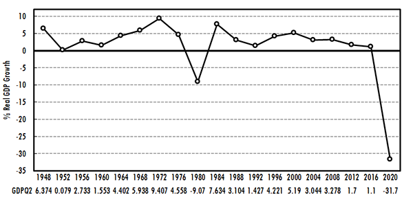
The second quarter 2020 economy presents several forecasting problems, even when truncated to -3% for diminishing effects (as 1980 was). First, to a much greater extent than in other attribution of responsibility cases, economic conditions in this case were dictated by the overwhelming bipartisan consensus to shut down the economy in order to stem the spread of the deadly pandemic, and not by the economic policies of the incumbent. Although there were some who favored less stringent precautions, with little knowledge of how best to limit the virus’s death toll, most agreed that a general shutdown of the non-essential economy was required. Under these circumstances, and given the healthy state of the pre-pandemic economy, it is hard to imagine anyone but the most partisan of Democrats blaming President Trump for the second quarter economic collapse. Moreover, unlike normal election years, GDP growth in the third quarter will not be anything like the catastrophic second quarter. Current projections of third quarter GDP growth range from around +19% to over +30%.[1]
So how should the economic predictors in the forecast models be treated in 2020? Should they just be set aside as hopelessly contaminated by the pandemic or would this be unfairly letting President Trump off the hook? And can a decision about this be objectively determined? The approval ratings, both in general and with respect to handling the economy, provide a good deal of insight on this matter. If the electorate were blaming President Trump rather than the international pandemic for the poor election year economy, his job performance approval ratings should be dreadful, but they are not. His current presidential approval ratings are about 45%, right around the politically neutral point. More telling is that 50% of the public approve of President Trump’s job performance as it relates to the economy.[2] These are not remotely the numbers of a president widely blamed for a weak economy, much less a 31.7% nosedive in the economy.
The 2020 forecasts
These numbers make clear that, unlike past elections, using second quarter GDP growth to predict the 2020 presidential election would be more misleading than instructive about the election’s likely outcome. Our best possible systematic readings of the election’s outcomes under these circumstances is to treat the economy as if it did not matter or that it was politically neutral between Trump and Biden. For purposes of distinguishing between incumbent and successor candidates in how voters apportion credit for economic conditions, I estimated the politically neutral growth rate for forecasts of past elections to be about 2.5%.
The estimated Trial-Heat and Convention Bump equations along with their preference poll only versions (assuming the economy does not matter) are presented in Table 1. The Trial-Heat (with GDP for estimation purposes) equation indicates that with Trump’s two-party standing of 46.2% in the Sept. 4 RealClearPolitics preference poll average (Biden 49.6% to Trump 42.6%, 60 days before Election Day) and assuming a neutral economic growth rate (GDP index = 0), he is predicted to receive 49.1% of the two-party national popular vote. A second Trial-Heat equation, dealing with the economic indicator by simply excluding it from the model, yields a 49.2% predicted two-party vote for Trump.
Table 1: Trial-Heat and Convention Bump Forecasting Models for the 2020 Presidential Election, 1948-2016
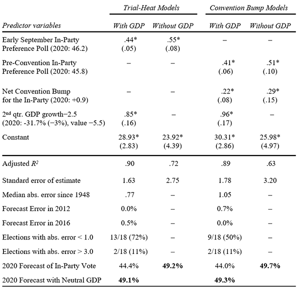
Notes: N = 17. *p<.01, one-tailed. Standard errors are in parentheses. The Durbin-Watson statistics ranged from 2.32 to 2.47. As in the past, 2008 was not included in the estimations since the unanticipated financial meltdown intervened between the forecast and the election. Also, as in the past, shrinking real GDP was truncated in recognition of diminishing marginal losses. The minimum is set at -3.0%. This comes into play in 1980 and this year. For 2020, this means the GDP value was −5.5% (−3.0−2.5=−5.5). Also with respect to GDP, it is scored as half-credit (or blame) for successor (non-incumbent) candidates (not applicable in 2020). A politically neutral economy is assumed to be a GDP growth rate of 2.5%.
The Convention Bump equations are also calculated with the assumption of a neutral economy and without the economic index produce similar predictions. With Trump’s standing in the RealClearPolitics polls of 45.9% of the two-party vote before the Democratic Party’s virtual convention (Aug. 17, Biden 50.2% to Trump 42.5%) and 46.7% after the Republican Party’s virtual convention (Sept. 1, Biden 49.0% to Trump 43.0%), the Convention Bump equations adjusted the two ways for the economic indicator problem predict a 49.3% and a 49.7% two-party popular vote for President Trump.
For the sake of the record and for complete transparency, Table 1 also presents what the forecast equations would predict for 2020 if the second quarter GDP numbers actually reflected the horrendous economic conditions (-3.0% circuit-breaker applied) for which the electorate was actually holding President Trump fully responsible — two demonstrably unreasonable assumptions. But if the violations of these assumptions were ignored, if voters acted like the robots they are sometimes made out to be, the outlook would have been a 56% or 55.4% Biden popular vote.
Conclusion
The forecasts, taking into account the economic indicator’s problem this year, indicate that the national popular vote division should be very close. The four versions of the forecasts are quite consistent in predicting an even narrower popular vote margin for Democratic candidate Joe Biden than Hillary Clinton received in 2016 when she won the popular vote, but lost the electoral vote. The electoral vote division in 2020 could easily go either way. With such a close election, our overheated political climate and the controversies sure to follow the additional adoptions of mail-in balloting as well as the many highly anticipated campaign events to come, the whole nation may be on blood pressure medication before this is over.
And, lest we forget, there are a number of nearly equally brutal congressional races to be decided and with them the partisan control of the House and Senate. My “Seats-in-Trouble” forecasting models based on the Cook Political Report’s handicapping of congressional contests in mid-August predicts Democrats to gain five seats and with them majority status in the Senate and predicts Republicans to gain five seats in the House — but we should not be too surprised if the likely turbulence of the presidential contest in the remaining weeks reverberates into some of these congressional races as well.
Do they make Maalox in red and blue?
| James E. Campbell is a UB Distinguished Professor of Political Science at the University at Buffalo, SUNY. His book, Polarized: Making Sense of a Divided America (Princeton, 2016), was named one of Choice’s Outstanding Academic Titles and is now available in paperback. |
Footnotes
[1] The 19.1% real GDP growth rate projection is the Aug. 14, 2020 median forecast of The Survey of Professional Forecasters for the Federal Reserve Bank of Philadelphia. The 30.8% projection is the Atlanta Fed GDPNow’s Sept. 10, 2020 estimate for the Federal Reserve Bank of Atlanta.
[2] The general 44.9% presidential approval rating and the public’s 50.4% approval of the president’s job performance with respect to the economy are the RealClearPolitics’ poll averages on Sept. 13, 2020.